RG #110: 3D scatter plot with multiple series in Y axis

X = seq(1, 100, 5)
Y = seq (1, 100, 5)
Z = rnorm (length (X), 10, 2)
data1 <- data.frame (X, Y, )
data2 <- data.frame (X, Y, Z1 = Z - 5)
data3 <- data.frame (X, Y, Z1 = Z - 3)

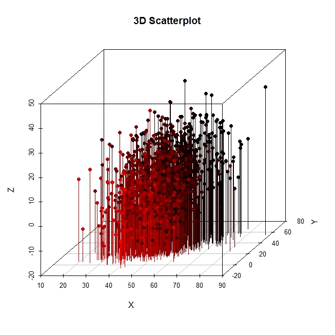
require(scatterplot3d)
s3d <- scatterplot3d(data1, color = "blue", pch = 19, xlim=NULL, ylim=NULL, zlim= c(0, 20))
s3d$points3d(data2, col = "red", pch = 18)
s3d$points3d(data3, col = "green4", pch = 17)

 

RG#107: Plot 3d horizontal lines (bars) over map (world and US example)

library("maps")
require(ggplot2)
library(ggsubplot)
world.map <- map("world", plot = FALSE, fill = TRUE)
world_map <- map_data("world")
require(lattice)
require(latticeExtra)

 # Calculate the mean longitude and latitude per region (places where subplots are plotted)

library(plyr)
cntr <- ddply(world_map,.(region),summarize,long=mean(long),lat=mean(lat))


# example data
 myd <- data.frame (region = c("USA","China","USSR","Brazil", "Australia","India", "Nepal", "Canada",
                                "South Africa", "South Korea", "Philippines", "Mexico", "Finland",
                                 "Egypt", "Chile", "Greenland"),
               frequency = c(501, 350, 233, 40, 350, 150, 180, 430, 233, 120, 96, 87, 340, 83, 99, 89))



subsetcntr  <- subset(cntr, region %in% c("USA","China","USSR","Brazil", "Australia","India", "Nepal", "Canada",
                                "South Africa", "South Korea", "Philippines", "Mexico", "Finland",
                                 "Egypt", "Chile", "Greenland"))

simdat <- merge(subsetcntr, myd)
colnames(simdat) <- c( "region","long","lat", "myvar" )


panel.3dmap <- function(..., rot.mat, distance, xlim,
     ylim, zlim, xlim.scaled, ylim.scaled, zlim.scaled) {
       scaled.val <- function(x, original, scaled) {
      scaled[1] + (x - original[1]) * diff(scaled)/diff(original)
     }
       m <- ltransform3dto3d(rbind(scaled.val(world.map$x,
           xlim, xlim.scaled), scaled.val(world.map$y, ylim,
          ylim.scaled), zlim.scaled[1]), rot.mat, distance)
        panel.lines(m[1, ], m[2, ], col = "green4")
      }


p2 <- cloud(myvar ~ long + lat, simdat, panel.3d.cloud = function(...) {
         panel.3dmap(...)
          panel.3dscatter(...)
 }, type = "h", col = "red", scales = list(draw = FALSE), zoom = 1.1,
            xlim = world.map$range[1:2], ylim = world.map$range[3:4],
          xlab = NULL, ylab = NULL, zlab = NULL, aspect = c(diff(world.map$range[3:4])/diff(world.map$range[1:2]),
          0.3), panel.aspect = 0.75, lwd = 2, screen = list(z = 30,
          x = -60), par.settings = list(axis.line = list(col = "transparent"),
            box.3d = list(col = "transparent", alpha = 0)))
 
print(p2)

# Over US map
library("maps")
state.map <- map("state", plot = FALSE, fill = FALSE)
require(lattice)
require(latticeExtra)

 # data
 state.info <- data.frame(name = state.name, long = state.center$x,
      lat = state.center$y)

set.seed(123)
state.info$yvar<- rnorm (nrow (state.info), 20, 5)


panel.3dmap <- function(..., rot.mat, distance, xlim,
     ylim, zlim, xlim.scaled, ylim.scaled, zlim.scaled) {
       scaled.val <- function(x, original, scaled) {
      scaled[1] + (x - original[1]) * diff(scaled)/diff(original)
     }
       m <- ltransform3dto3d(rbind(scaled.val(state.map$x,
           xlim, xlim.scaled), scaled.val(state.map$y, ylim,
          ylim.scaled), zlim.scaled[1]), rot.mat, distance)
        panel.lines(m[1, ], m[2, ], col = "grey40")
      }

pl <- cloud(yvar ~ long + lat, state.info, subset = !(name %in%
       c("Alaska", "Hawaii")), panel.3d.cloud = function(...) {
         panel.3dmap(...)
          panel.3dscatter(...)
 }, col = "blue2",  type = "h", scales = list(draw = FALSE), zoom = 1.1,
            xlim = state.map$range[1:2], ylim = state.map$range[3:4],
          xlab = NULL, ylab = NULL, zlab = NULL, aspect = c(diff(state.map$range[3:4])/diff(state.map$range[1:2]),
          0.3), panel.aspect = 0.75, lwd = 2, screen = list(z = 30,
          x = -60), par.settings = list(axis.line = list(col = "transparent"),
            box.3d = list(col = "transparent", alpha = 0)))
 print(pl)

RG#99: cloud 3D bars with heatmap

require(lattice)

require(latticeExtra)

data(VADeaths)

cloud(VADeaths, panel.3d.cloud = panel.3dbars,
      xbase = 0.4, ybase = 0.4, zlim = c(0, max(VADeaths)),
      scales = list(arrows = FALSE, just = "right"), xlab = NULL, ylab = NULL,
      col.facet = level.colors(VADeaths, at = do.breaks(range(VADeaths), 20),
                               col.regions = cm.colors,
                               colors = TRUE),
      colorkey = list(col = cm.colors, at = do.breaks(range(VADeaths), 20)),
      screen = list(z = 40, x = -30))

RG# 55: 3D plots (scenes) from data points

# data 
x <- seq(-2,2,len=100)
grd <- expand.grid(x = x, y = x, z = x)
arv <- array(grd$x^2 + grd$y^2 + grd$z^4, rep(length(x),3))


require(misc3d)
cnn <- computeContour3d(arv, max(arv), 1)
drawScene(makeTriangles(cnn))

#volcano plot 
data(volcano)


 voldf <- local({
zz <- 7 * volcano
xx <- 20 * (1:nrow(zz))
yy <- 20 * (1:ncol(zz))
surfaceTriangles(xx, yy, zz, color="cyan2")
})
drawScene(voldf, scale = FALSE)

RG#46: 3D-spinning scatter plots

set.seed(12444)
X = rnorm (1000, 50, 10)
Y = X*0.6+rnorm(length(X), 0, 10)
Z = Y*0.3+ +rnorm(length(X), 0, 10) 

# using rgl package 

library(rgl)

plot3d(Z, X, Y, col="red", size=3)

# another using package Rcmdr 

library(Rcmdr)

scatter3d(Z, X, Y)

RG#45: 3D scatter plots (with vertical lines and regression line)

set.seed(12444)
X = rnorm (1000, 50, 10)
Y = X*0.6+rnorm(length(X), 0, 10)
Z = Y*0.3+ +rnorm(length(X), 0, 10) 


# 3D Scatterplot
require(scatterplot3d)
scatterplot3d(X,Y,Z, pch = 19, color = "green4", main="3D Scatterplot")

thdp <- scatterplot3d(X,Y,Z, pch = 19,  main="3D Scatterplot", highlight.3d=TRUE,
type="h")

fitm <- lm(Z ~ X+Y) 
thdp$plane3d(fitm)

trdt <- scatterplot3d(X,Y,Z, pch = 19, color = "green4", main="3D Scatterplot")
trdt$plane3d(fitm)

require(lattice)

cloud(Z~X*Y,main="3D Scatterplot", pch = 18, col = "green4", scales = list(arrows = FALSE)) 

RG#31: 3D- Explodated pie chart

# data
slices <- c(18, 12, 4, 16, 8, 9, 12)
lbels <- c("US", "UK", "Australia", "Germany", "Canada", "India", "China")


# plot
library(plotrix)
pie3D(slices,labels=lbels,explode=0.1, main="3D- explodated Pie Chart")

 

RG#14: 3D plot - wireframe plot

 # data
XV <- seq(-4, 4, len = 40)
 YV <- seq(-4, 4, len = 40)
datf <- expand.grid(xvar = XV, yvar = YV)
 datf$ZV<-  datf$xvar^2 + datf$yvar^2 - 2*datf$xvar* datf$yvar

# plot
require(lattice)
wireframe(ZV ~ xvar* yvar, data = datf)

wireframe(ZV ~ xvar* yvar, data = datf, drape = TRUE, perspective = FALSE, aspect = c(3,2), colorkey = TRUE)